Version 24 new features and enhancements
Version 24 provides new facilities and improvements for modelling cables, joints and interfaces, piles and anchors, for defining carriageways. It also introduces a new smart combinations and envelopes facility, improved design combinations and two more geotechnical models.
In detail...
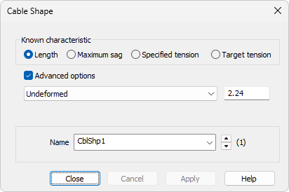
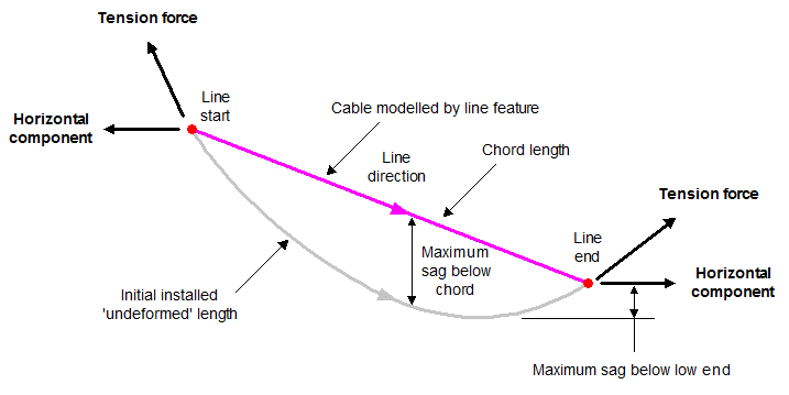
Improved modelling of cables
- Cable (catenary) elements and Cable (Ernst) elements are now available. They are used in conjunction with Cable shape attributes, which determine the reference configuration of a cable after it has been added to a structure. The initial (sagged) shape of the cable can be determined using an unstressed length, a maximum sag, or a specified or target tension force. The use of Cable (Ernst) elements also requires the use of Cable (Ernst) material.
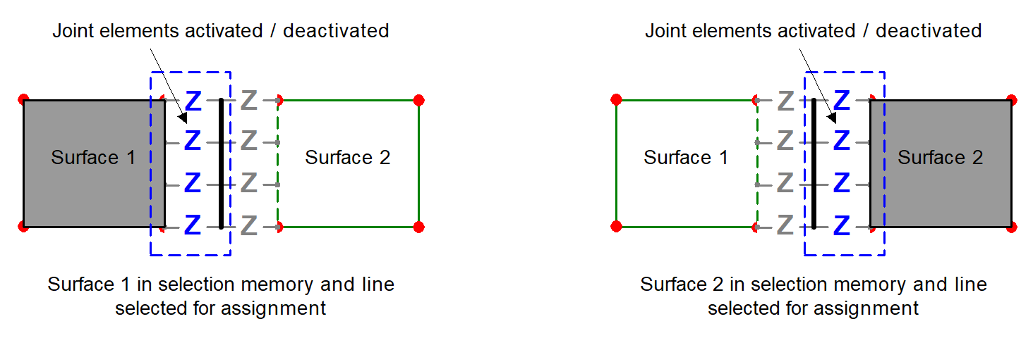
Improved activation and deactivation of joint and interface elements
- Much greater control is now provided over which elements an activate / deactivate assignment applies to, in the case of single feature and interface pairing mesh assignments.
- When assigning and deassigning activate and deactivate attributes to and from selected features, other features may be added to selection memory to clarify to which set of joint/interface elements the activate / deactivate assignment applies. The joint / interface elements that are connected between the main selection and selection memory will receive the activation / deactivation.
Single feature assignment of joints and interfaces for connected geometry
- Single feature meshing can now be used to model a common situation in soil-structure interaction modelling where a retaining wall is tied back into the ground, no longer requiring the use of coincident geometry and interface pair meshing, as is shown in the 2D model image below.
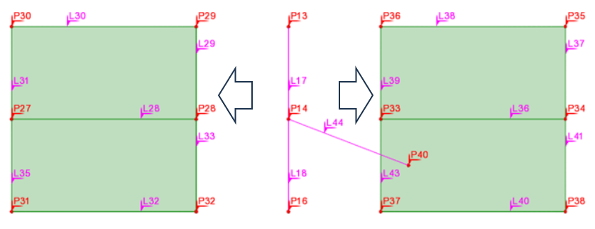
Exploded view of a pre-version 24 model showing two lines modelling a wall, isolated by joints (not shown), tied-back into the ground, between two pairs of surfaces modelling the ground. All coincident lines are set to be unmergeable.
For the 2D model below, the retaining wall is modelled in Version 24 without any coincident features:
- Beam elements are assigned to lines 29, 33 and 44
- Surface elements are assigned to all surfaces
- Single feature joint assignments are made to line 29 and line 33 representing the wall to isolate them using interface elements from the surfaces either side.
- Line 44 representing the ground anchor will remain only connected to lines 29 and 33 (and not to other lines in surfaces connecting at that point) because, in this scenario, a feature will only connect to a feature of the same type (e.g. a line to a line, a surface to a surface).
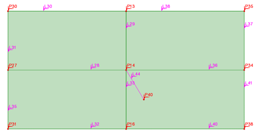
Version 24 model showing two lines modelling a wall, isolated by joints (not shown), tied-back into the ground, between two pairs of surfaces modelling the ground. All coincident lines are set to be unmergeable.
See Geotechnical / SSI interface for details of capabilities
Improved modelling of piles and rock anchors in continuum models
- Piles, soil anchors, or any similar devices that penetrate a soil continuum and attach to it by friction can now be modelled by embedding beam or bar elements within continuum elements without the need for the soil geometry and mesh that is modelling the continuum to be aligned with the pile geometry, making the modelling of piles in geotechnical analyses much easier. Appropriate materials and elements need to be assigned to line and point features modelling the pile to model the slip between the pile and the continuum.
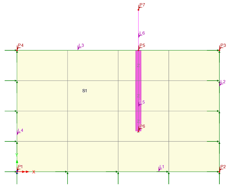
2D model showing fleshed thickness of pile
3D model
See Geotechnical / SSI interface for details of capabilities
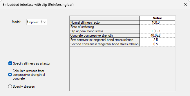
Modelling of bond slip based on CEB-FIP model code
- An embedded interface with slip (Reinforcing bar) material model has been added to model the slip between embedded reinforcing bars and the surrounding cementitious matrix, which plays an important role in the accurate prediction of crack widths, as well as ultimate load analysis when bond slip contributes to failure.
- Nonlinear interface laws are used to describe the bond stress-slip relationship with one law taken from the CEB-FIP model code, whilst the second, which can be considered a smoothed version of this, is the Popovic model. Both models enable the simulation of the nonlinear bond slip behaviour to be modelled.
Free Cantilever Method (FCM) Wizard enhancements
- The FCM wizard has been enhanced to permit generation of bridge models to any alignment by using a reference path. FCM wizard data held in the Bridge data entry in the Utilities Treeview can now be edited and models re-created.
- See
Free Cantilever Method (FCM) Wizard.

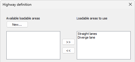
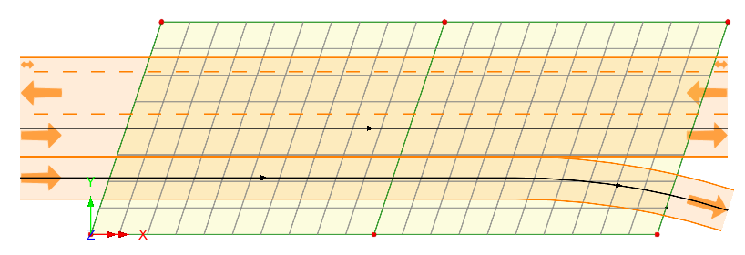
Improved carriageway definition and visualisation for traffic load optimisation
- The location of lanes in a carriageway can now be specified with reference to a centreline or other longitudinal line forming part of a bridge deck, rather than having to define lines representing kerbs to indicate the extent of a carriageway as was required prior to version 24.0. This greatly simplifies the definition of a carriageway and also now allows divergent carriageways to be loaded.
- Lanes within each carriageway can have different widths, and the direction of traffic within each lane can be specified.
- Visualisation of defined carriageways now shows their extent and the traffic direction specified, and feedback is given regarding the carriageways that are used in the Vehicle Load Optimisation runs.
AASHTO LRFD 10th edition now supported
- See
Vehicle Load Optimisation for all codes supported.
TRVINFRA-00331 (Sweden) now supported
- EN1991-2 Sweden 2023 is now supported and offers traffic load options in compliance with the TRVINFRA-00331 design standard. Separate sets of results can be produced for complimentary load (a), referred to as set 'EG A', and the most onerous one between (b) to (o), referred to as set 'EG B'. The implementation now allows for obtaining results for each load group in one VLO Run, without the need to create a VLO Run for each load group. The vehicle types j, k and l have been updated in accordance with Clause 8.3.2.2.1 in TRVINFRA-0331 so that the varying distance between the bogies can be greater than either 25m or 45m.
- See
Vehicle Load Optimisation for all codes supported.
Design of prestressed concrete structures - Eurocode 2
- The Eurocode 2 reinforced concrete design capability has been extended to include bonded post-tensioned prestressed concrete members, allowing engineers to perform reinforced concrete and prestressed design checks within a single, consistent workflow. Users now benefit from comprehensive ULS and SLS verification (including stress limitation, crack control, shear, and torsion) fully aligned with EN 1992, reducing the need for external tools and manual checks.
- See
RC frame design for more information.
Concrete frame design and RC slab / wall design now supports AASHTO 10th edition
- AASHTO 10th edition is now documented as being supported.
- See
RC frame design for and
RC slab / wall design more information.
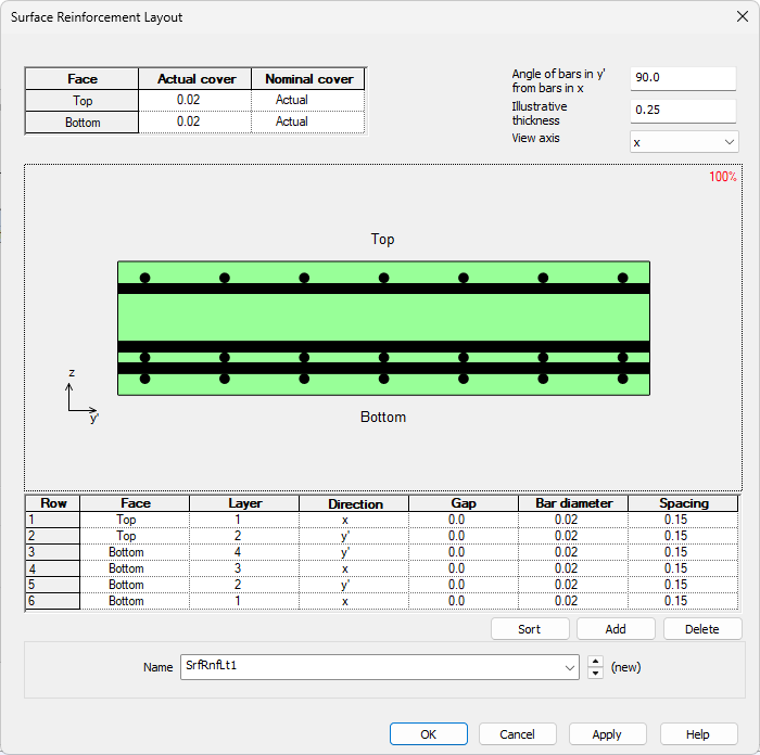
RC Slab / Wall design now supports multiple reinforcement layers
- Multiple reinforcement layers can now be defined in each face and sorted within the grid according to their face and layer number.
- See RC frame design for and RC slab / wall design more information.
Creep material updates for AS5100.5-2017 and NZS3101:2006
- The existing codified creep material models for AS5100.5-2017 and NZS3101:2006 have been updated to account for material properties prior to 28 days.
Creep and shrinkage for CSA S6:19 now supported
- See Prestress/post-tensioning for all codes supported.
Steel frame design calculations to CSA S6-14 and S6:19 are now faster
- Steel frame design checks are now faster, and in addition a Steel Frame Design loadcase / results container entry is now created in the Analyses Treeview, as opposed to the Utilities treeview, in keeping with the way that RC frame design results are created and accessed.
- See Steel frame design for the range of codes supported.
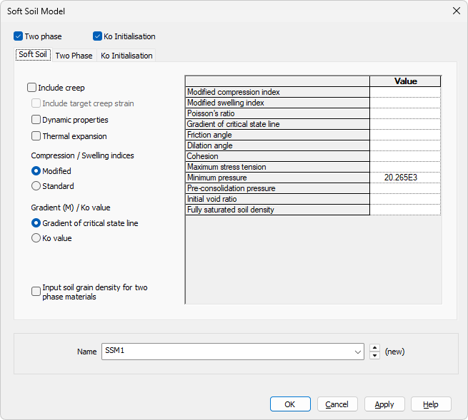
Soft Soil Material Model now provided
- The Soft Soil material model is suitable for materials with a high degree of compressibility such as lightly over-consolidated, near normally consolidated soft soils such as clays, clayed silts and peat undergoing primary compression. For soils that are less compressible, the Hardening Soil Model should be used.
- The model provides a cap to a Mohr Coulomb yield surface and incorporates the logarithmic compression behaviour similar to that often found in critical state models. Its parameters are obtained directly from standard triaxial and oedometer laboratory tests.
- See
Geotechnical / Soil-structure interaction for the range of soil models supported.
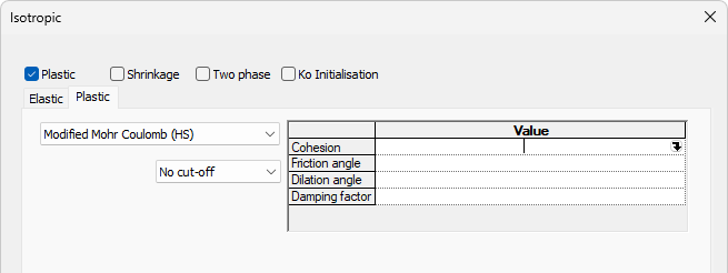
Modified Mohr-Coulomb (HS) model now provided
- The Modified Mohr-Coulomb (HS) model replaces the now superseded Modified Mohr-Coulomb model, which remains supported within the software allowing existing models that use it to tabulate and solve the same as they did in previous versions.
- The new model tabulates as a special case of the hardening soil model offering improved convergence.
- See
Geotechnical / Soil-structure interaction for the range of soil models supported.
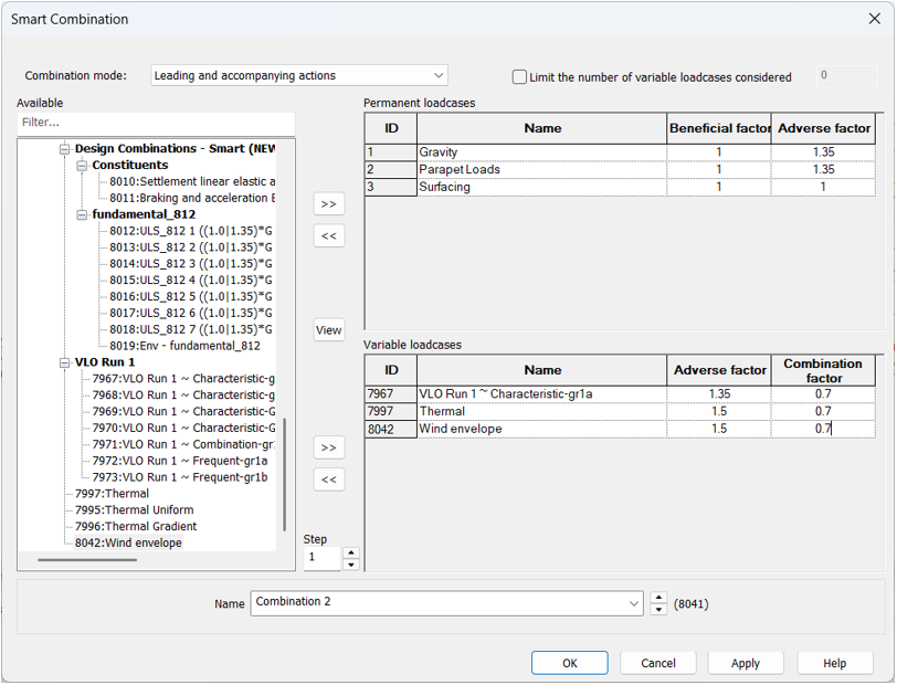
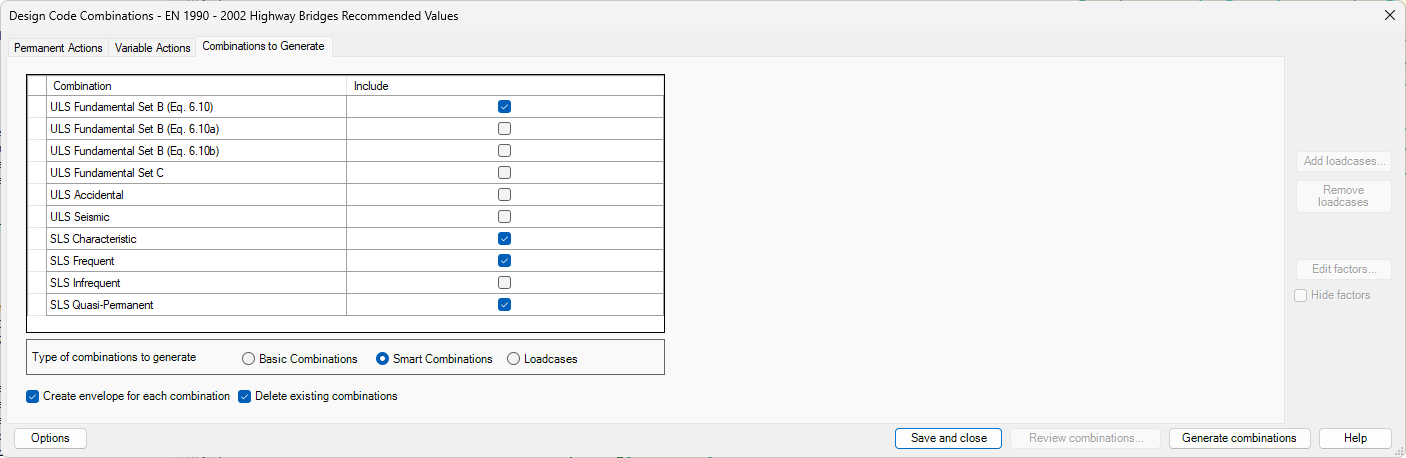
Improved smart combinations and envelopes facility
- Smart combinations have been replaced with new versions which provide an interface more familiar to bridge engineers and an option to apply leading and accompanying factors.
- The new combinations are represented with a single entry in the Analyses treeview, further simplifying their use. New envelopes have also been added to be compatible with this single entry approach.
In summary:
- Loadcases are now separated into permanent and variable within the smart combination dialog, which makes it clear to which loadcases the option 'Limit the number of variable loadcases' refers to.
- A new mode "Leading and accompanying actions" has been added, which aligns with the Eurocode approach of having a leading variable action with reduced effects of all other variable actions. This allows the leading variable action to be evaluated by the combination at each location, rather than having to create a combination for each leading variable action, as was required previously.
- The smart combination will sort all variable actions by their effect. The option "Limit the number of variable actions" will limit the number of effects considered, capturing the most onerous.
- When created, a single smart combination or envelope loadset is now added to the Analyses Treeview, as opposed to maximum and minimum loadsets as used previously. This contains both maximum and minimum results, which can be individually chosen when setting active a loadcase or printing or viewing results.
- Legacy versions of the smart combination and envelope facilities have been retained to support models created prior to version 24. Menu items for the legacy combinations and envelopes are only available if the model contains one or more combinations or envelopes. These are identified by the addition of the wording '(Legacy)' on their menu item names. Note that smart combinations and envelopes created in earlier software versions cannot be used inside a Version 24 smart combination or envelope and vice-versa because they are incompatible.
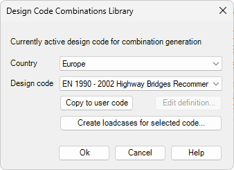
Improved design combinations facility
- The design combinations facility has been made generally easier to use and more flexible to select and review the combinations being created.
- More control is provided over how design combinations can be automatically generated.
- It is now also possible to author your own "design codes" for combinations and share them with others in your organisation. By taking an existing design code, you can make edits to suit regional or project requirements.
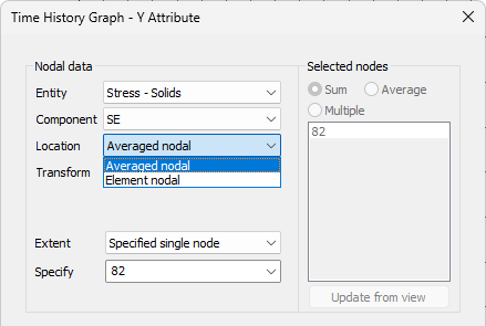
Graph wizard enhancements
- A 'Location' option has been provided in the graph wizard for nodal history. For "non-continuous" results (such as stresses or strains that are calculated on an element by element basis) the location options provide for:
- Averaged nodal results, where if a selected node is not on a discontinuity, a single curve is drawn as if it were continuous. If a selected node is on a discontinuity, as many curves are drawn as required to respect the boundary, whilst averaging connected element results where valid.
- Element nodal results (unaveraged), where one curve is drawn for each element connected to a selected node.
- A similar 'Location' option has also been added to the 'Slice data' dialog of the 'Graph through 2D' facility for the same purpose.
- Default titles are now added to the graph X and Y axes according to the selections previously made within the wizard.
- For time history graphs, the units to be used to plot the graph can be specified. This excludes nodal history graphs plotting a slideline or thermal surface entity.
- User-defined results can now be plotted for history graphs that don't use the slideline or thermal surface entity.
LUSAS GitHub repository
- Introduced between the releases of V22.0 and V23.0, the LUSAS GitHub repository provides practical examples of using the LUSAS Programming Interface (LPI) in Python, VBScript, Jupyter, C#, VB.Net and Grasshopper.
- The repository provides engineers with a centralised, well-documented set of automation examples using the LUSAS Programming Interface (LPI) and encourages the use of LUSAS in digital workflows (e.g., BIM, Python-based engineering, AI-assisted design) by lowering the learning curve.
See the LUSAS GitHub repository for more details.

New Grasshopper plugin components
- Point, Activate/deactivate, Volume member, Volume mesh, Loadcase, and Re-order loadcase components have been introduced into the LUSAS plugin for Grasshopper since the release of V22.0 and V23.0.

Python now supplied as part of a LUSAS installation
- An embedded Python interpreter is now provided as part of the LUSAS installation.
- It can be used to run Python scripts from LUSAS and, when 'Python' is selected as the script language in the LUSAS configuration utility it will be used to generate session files and display LPI commands in the Python language.
See LUSAS Programmable Interface (LPI) Scripts for more information
User manuals
- Relevant documentation has been updated for this new release.
- Selected manuals are provided in PDF format as part of the LUSAS installation and are also available for download from the LUSAS website.
Worked examples
Step-by-step, overview and verification examples, and associated files referenced by those examples are available for download from the User Area of the LUSAS website. New for this release are:
- Worked example: Erection of a cable-stayed cantilever structure.
- Geotechnical overview examples: Axially loaded pile, Braced sheet pile, Pile raft foundation, Pile bridge foundation
- Geotechnical verification example: Rigid strip footing on soft soil.